Superalgos/docs/pages/suite/suite-build-a-plotter.md

title, summary, sidebar, permalink

title	summary	sidebar	permalink
Build a Plotter		suite_sidebar	suite-build-a-plotter.html

Introduction

A plotter is a device used to produce a graphic representation of the data generated by indicators. They usually have a one-to-one relationship with indicators, as they are often created as a customized solution.

However, in practice, there is no constraint to creating any number of plotters for a single indicator or a single plotter for multiple indicators.

This page takes you through the process of creating a plotter. for further reference, feel free to explore the following list of plotters that ship with the app:

• Team Masters: Plotters-Bollinger-Bands, Percentage B module.

• Team Sparta: SMA, RSI and EMA, all modules.

Team	Plotter

Plotters are created at the root of the Teams hierarchy and have the most basic configuration:

{
"codeName": "Plotter Name"
}

Plotter Module

Plotter	Plotter Module

A plotter module is a device within a plotter that contains the definitions to create the visualization for a particular layer populating the Layers Panel in the Charts.

A single plotter may have several modules. You may choose to use different modules to plot each product of the indicator, or as best suits the expected use-pattern.

In cases in which the module's job is to render graphics directly over the same price scale used by candles (i.e.: Moving Averages, Bollinger Bands, etc.), then its configuration is very simple:

{
"codeName": "Plotter-Name",
"banner": "Band"
}

In other cases, you will want to render information on a different scale, for example, in the case of oscillators (i.e.: Relative Strength Index, Percentage Bandwidth, etc.). For such cases, you will use the following type of configuration:

{
    "codeName": "Plotter-Name",
    "slot":  {
        "number": 3,
        "minValue": 0,
        "maxValue": 100
    },
    "banner": "Oscillator"
}

• codeName is the name used in the code to refer to the module.

• slot, number is an integer from 2 to 11, 2 representing the top-most section of the screen and 11 the bottom-most section.

• slot, minValue is the minimum possible value of the scale (for example, 0 for RSI).

• slot, maxValue is the maximum possible value of the scale (for example, 100 for RSI).

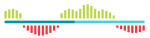
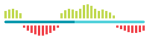
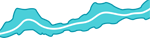
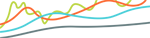
• banner is the name of the image that illustrates the corresponding layer in the Layers Panel. In case the banner is not specified, the default banner is used. Current possible values are:

Value	Image
Default
Histogram
Band
Moving Average
Oscillator
Trend

You may also add and use your own images. To do that:

1. name your image in the following format: Your-Image-Banner.png;

2. place your images in the WebServer\Images\ folder;

3. in the configuration of the module, use the name without the -Banner ending (e.g.: "banner": "Your-Image")

Beyond the module's configuration, the most important aspect of a module's behavior is obtaining data from bot's products. For a module to be able to obtain data from a certain product, you need to link the said product to your module.

Shapes

Plotter Module	Shapes

The shapes node contains all of the definitions required to render graphics on the screen.

A plotter recursively renders graphics for each period (or candle). This means that you will define—in generic terms—what shapes need to be drawn for a single period, and the plotter will do the same thing for every candle that is visible on the screen at any point in time, for any time frame, as long as the corresponding data is available.

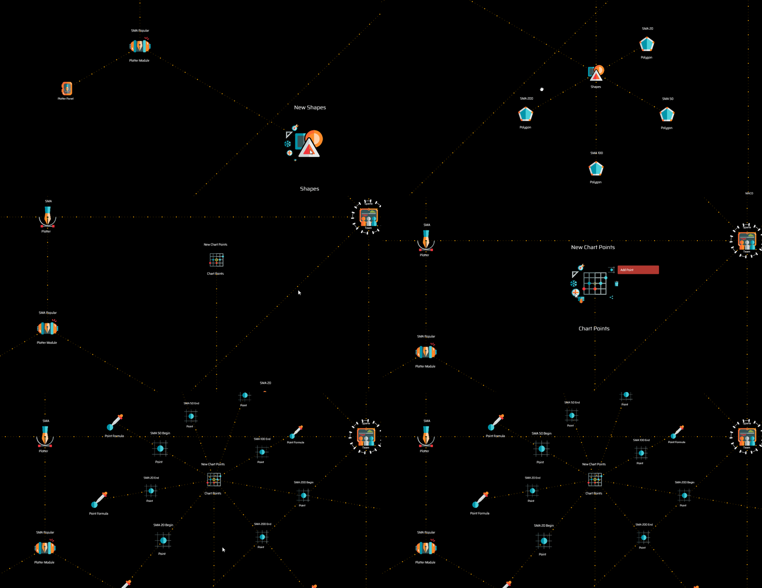
In general terms, the process of defining what is going to be rendered on the screen consist of the following four steps:

1. Identifying points defined by [x,y] coordinates

Points Chart	Point	Point Formula

Add a points chart node to define the points you will use. The points are ultimately defined by their point formulas.

In the case you wish to represent some form of variation of the price over time, then a typical point formula consists of the following two coordinates: x = datatime and y = rate.

For example:

Point SMA 20 Begin

x = record.begin
y = record.previous.sma20

The example above shows the definition of the first of two points necessary to draw the segment of the 20-periods SMA curve for any particular period or candle. In this case, x = record.begin is the starting datetime of the period (or candle) and y = record.previous.sma20 is the rate of the 20-periods SMA of the previous candle.

NOTE: Make sure you give each point a significant name, as you will later need to reference them when you define the styles of the polygons you are drawing.

To complete the line segment corresponding to a single candle, you will need the closing datetime of the candle and the closing rate for the 20-periods SMA:

Point SMA 20 End

x = record.end
y = record.sma20

The above system works very well for plotting all sorts of information over the candles, on the charts.

Let's see what happens when instead of plotting graphics directly over the candles, you are building, for example, an oscillator.

An oscillator like RSI will too need the definition of the starting and ending datetime of the period as the value for the x-axis. However, the value for axis y will fit the scale defined on the plotter module configuration.

Anyway, the points definition is just as straight forward, for example:

Point RSI Begin

x = record.begin
y = record.previous.value

Point RSI End

x = record.end
y = record.value

The chart points you define on this first step may be used as many times as you may need for as many polygons as you wish. For example, the current RSI 14 plotter module features the following four points:

Point Begin 20

x = record.begin
y = 20

Point End 20

x = record.end
y = 20

Point Begin 30

x = record.begin
y = 30

Point End 30

x = record.end
y = 30

Those four points are later used to paint the background of the RSI 20 to 30 value range of the RSI chart slot. The first two points are also used to draw the dotted line that signaling the 20-value mark, and the last two are used for the dotted line indicating the 30-value mark.

2. Defining polygons

Polygon	Vertex

The first few nodes that define a polygon are its vertices. All you need to do to define the vertices of a polygon is to create them and establish a reference to the corresponding chart points you previously defined.

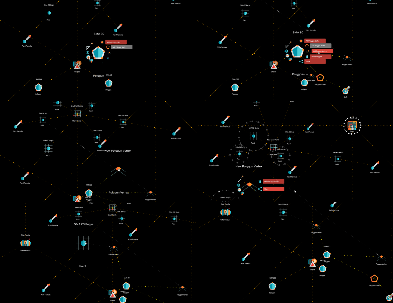
As stated earlier, for drawing curves you will need two vertices. For painting the background of a chart, you will likely need four.

NOTE: Bear in mind that the order in which you create the vertices in a polygon, or actually, the final order in which they are arranged around the parent polygon node when their rotational symmetry property is selected, is the order in which the plotter will compute the points. This means that, if you are drawing a box, you need to make sure the points are ordered appropriately. Imagine you need to draw a box on a piece of paper without lifting the pencil... that is how the plotter will do it.

You may define as many polygons as you need.

NOTE: The order in which polygons are ordered around the parent shapes node determines the order in which they are drawn on the screen. If you have intersecting polygons, those drawn last will be drawn on top of those drawn first.

3. Defining default styles

Now that your polygons are mathematically defined, all that is left is defining their style. To do that, you have the following nodes available:

Polygon	Body	Border	Style

You will create a body node when you wish to create a fill for a closed polygon of at least three vertices.

You will create a border node when you wish to create a stroke for the outlines of any sort of polygon, either closed or open.

Both of these nodes feature the option to add a style. When you add a style to a body or border node, the style acts as the default style.

A typical definition for a body node looks like this:

{
    "default": {
        "opacity": 0.2,
        "paletteColor": "UI_COLOR.DARK_TURQUOISE"
    },
    "atMousePosition": {
        "opacity": 0.3,
        "paletteColor": "UI_COLOR.DARK_TURQUOISE"
    }
}

A typical definition for a border node has a couple more properties:

{
    "default": {
        "opacity": 0.2,
        "lineWidth": 1,
        "lineDash": [0,0],
        "paletteColor": "UI_COLOR.DARK_TURQUOISE"
    },
    "atMousePosition": {
        "opacity": 0.3,
        "lineWidth": 2,
        "lineDash": [0,0],
        "paletteColor": "UI_COLOR.RUSTED_RED"
    }
}

The first section of the definition refers, as explicitly stated, to the default state of the style.

The second section refers to the style assigned to the column or period on which the mouse pointer is located. This is very useful for highlighting the specific zone of interest as the user browses the charts.

• opacity is probably self-explanatory: it may range from 0 for a fully transparent object to 1 for a solid object.

• paletteColor sets the color for the fill or stroke in cases of polygon bodies and polygon borders respectively. Use the variable UI_COLOR followed by a . and any of the properties in the following list for a selection of currently available colors:

Variable Value	RGB Value
DARK	48, 48, 54
LIGHT	234, 226, 222
GREY	150, 150, 150
LIGHT_GREY	247, 247, 247
WHITE	255, 255, 255
BLACK	0, 0, 0
GOLDEN_ORANGE	240, 162, 2
RUSTED_RED	204, 88, 53
GREEN	188, 214, 67
RED	223, 70, 60
PATINATED_TURQUOISE	27, 153, 139
TITANIUM_YELLOW	244, 228, 9
MANGANESE_PURPLE	91,80, 122
TURQUOISE	74, 207, 217
DARK_TURQUOISE	2, 149, 170

• lineWidth is the width of the border line, which should be greater than 0.

• lineDash is used to turn the border into a dashed-line; the first value corresponds to the length of the dash while the second value defines the length of the space.

NOTE: When using dashed lines, bear in mind that the drawing from one column or period is independent of the next. Big values for dashes and spaces may not work well for lines that span several columns.

4. Defining conditional styles

A great way to introduce additional intelligence on the visual representation of data is to use styles that respond to certain conditions.

For example, the Percentage Bandwidth plotter module assigns a different color to the Moving Average line when it's going up than to when it's going down.

To do that, after defining the default style, you may select Add Style Condition from the body or border node menu.

Style Condition	Style

Style conditions work pretty much like conditions you use on your trading systems. The main difference is that the variables available are solely those provided by the indicator products that may be linked to the plotter.

To continue the example of the Percentage Bandwidth plotter, the following is the condition that determines the newly added styles:

record.previous.movingAverage > record.movingAverage

As hinted earlier, when the condition is met, the default style is modified by a second style that may be created on the menu of the style condition node.

The definition of secondary styles is slightly different from that of the default style, as—in such cases—you may no longer define the atMousePosition property:

{
    "opacity": 0.55,
    "lineWidth": 1,
    "lineDash": [0,0],
    "paletteColor": "UI_COLOR.RED"
}

You may define as many style conditions as you wish. The system evaluates all style conditions in a sequential order determined by their position in the rotational symmetry around the parent node.

Each condition that is met may modify or add up to the resulting style that is rendered on screen. That is, the final style is the result of the sequential application of the styles defined for each condition that is met, on top of the default style.

Panels

Beyond the graphic representation of data over the charts, plotters may also feature a data panel, that is, a numerical representation of the data showing the exact figures corresponding to the column or period that is in focus (the point of the charts where the mouse pointer is at any point in time).

Panel	Panel Data	Data Formula

Once you select Add Plotter Panel on the plotter module menu, you may start adding as many data fields as you wish.

The system will render a panel featuring a centered, single-column vertical arrangement of data. The label of each data field on the panel is given (by default) by the label you set for the panel data node.

The configuration of a panel data node allows you to determine the number of decimal places for the corresponding data field:

{
    "valueDecimals": 2
}

If you wish to override the default manner in which the data is assembled on the panel, you may include and define the following properties:

{
    "labelText": "Your Label",
    "labelPosition": 15,
    "valuePosition": 20,
    "valueDecimals": 2
}

• labelPosition and valuePosition represent the vertical distance of the corresponding field with the top margin of the panel.